Moment of inertia of a uniform triangle about an axis through its center of mass

Introduction:
In this activity, we were trying to find the moment of inertia of an uniform triangle, and it was being rotated about an axis through its center of mass.

Apparatus and steps:

1.The Pasco rotational sensor was connect to the computer, and we first let it rotate with the smaller topper disk with a hanging mass and no other mass attached to the rotating disk.
The logger pro would record the angular speed and angular acceleration, and they would help us found the moment of inertia of the rotating disk.

2.Then we attached the triangle through its center of mass on the rotating disk, and collect its angular speed and angular acceleration.

3. Finally, we spin the triangle so the longer side of the triangle was horizontal to the ground, and we let it rotate to collect its angular speed and angular acceleration.















Data and analysis:
1.The rotation motion of the pasco rotational sensor without the triangle:

The α(down)=2.278 rad/s^2, α(up)=2.104 rad/s^2

2.The rotation motion of the pasco rotational sensor with the triangle(shorter side at the bottom):

The α(down)=2.102 rad/s^2, α(up)=1.943 rad/s^2

3. The rotation motion of the pasco rotational sensor with the triangle(longer side at the bottom):

The α(down)=1.938 rad/s^2, α(up)=1.735 rad/s^2

The following are the steps to obtain the calculated inertia:

The following are the steps to obtain the theoretical inertia:

The theoretical values of the moment of inertia is almost the same as the ones we calculated with the experimental data collected, the small % error are very likely to be caused by the friction in the system.

Meter stick with Clay

Introduction:
In this activity, we released the ruler from a certain height, and we predicted the maximum height it would reach by calculation. Then, we use logger pro to measure the actual maximum height it would reach.

Apparatus:

A clay was placed at the bottom of the ruler's path.

The top of the ruler was
stabled on the motion
sensor.















Prediction made with calculation:

We predicted the maximum height the clay would reach in the motion to be 0.336 m from the ground.

The actual height found with logger pro:

From the Logger Pro, we could find the maximum height that the meter stick and the clay could reached is 0.1312m.
%error = (0.336-0.1312)/0.336 *100% =60%

Conclusion:
The difference between the calculated prediction and the actual height measured by the logger pro is very large. The large difference might be caused by the friction between the clay and the ground. Because the clay is sticky, a lot of energy was lost trying to separate the clay and the ground. Since we predict the maximum height under ideal condition when it was really not ideal. To make an more accurate prediction, we should take the air resistance, the stickiness of the clay, and the friction on the pivot point.

Angular acceleration

Introduction:
The purpose of this lab is to figure out the angular acceleration of object with known torque, and determine which factor would affect the angular acceleration the most: The magnitude of the force that creates torque, the radius of the spinning object, or the mass of the rotating object.
To fulfill the goals above, we did three types of experiments:
Experiment 1,2 and 3: Effect of changing the hanging mass
Experiment 1 and 4: Effect of changing the radius and which the hanging mass exerts a torgue
Experiment 4,5,6: Effect of changing the rotating mass

Apparatus:

   The rotating disk was placed on another disk with air blowing between them to create an almost frictionless surface of rotation.
   We would be able to change the rotating radius by attaching the string at inner or outer radius of the disk, and we could change the weight of the hanging mass, and we could also change the rotating mass by place different hanging mass on the rotating mass.
   The rotating system was connected to a computer so we could use logger pro to collect the angular acceleration.









The following stats are the different radius, masses we used in the experiment:

Data and Data Analysis:
Experiment 1:
(Hanging mass: 0.0245 kg; small torque pulley; top steel disk rotating)

We obtained that: α(down)=1.083 rad/s^2, α(up)=1.192 rad/s^ 2


Experiment 2:
(hanging mass: 0.050kg; small torque pulley; top steel disk rotating)

We obtained that: α(down)=2.083 rad/s^2, α(up)=2.500 rad/s^ 2

Experiment 3
(hanging mass: 0.075kg; small torque pulley; top steel disk rotating)

We obtained that: α(down)=2.597 rad/s^2, α(up)=4.328 rad/s^ 2

Experiment 4:
(hanging mass: 0.0245kg; large torque pulley; top steel disk rotating)

We obtained that: α(down)=2.110 rad/s^2, α(up)=2.316 rad/s^ 2

Experiment 5:
(hanging mass: 0.0245kg; large torque pulley; top aluminum rotating)

We obtained that: α(down)=5.955rad/s^2, α(up)=6.214 rad/s^ 2

Experiment 6:
(hanging mass: 0.0245kg; large torque pulley; top steel disk and bottom steel disk rotating together)

We obtained that: α(down)=0.7944rad/s^2, α(up)=1.562 rad/s^ 2

We organized the above collected data into the following table:

Conclusion:
As a result, we found that the angular acceleration to be directly proportional to the hanging mass when other conditions are the same; the angular acceleration is directly proportional to the radius the torque was applied to when other conditions are the same; the larger the rotating mass is, the smaller the angular acceleration will be when other conditions are the same.

Momentum and energy in two- dimensional collision

Introduction:
The purpose of this lab is to understand how momentum and energy change in two dimensional collision.

Apparatus:

The bottom plate was where we collide the balls, and all the balls could roll without slipping on the plate. Above the plate was an camera that would capture the motion of all the balls before and after collision.
The video of the balls' motion was recorded into our computer, and we used logger pro to create velocity vs. time graph corresponded to the video.

The following is an example of how we pin the position of the balls at every instant:












Data and Data Analysis:

Steel balls collision

The following is the position vs. time graph of the collision of metal balls (small steel ball's mass=10.38g; big steel ball's mass=28.78g)

We can simply find the velocity of two balls before and after collision by find out the slope of the position functions of time.
Before the collision, 28.7g steel: Vx=0.6107m/s Vy=0.007932m/s
After the collision,  28.7g steel: Vx=0.006845m/s, Vy=0.2147m/s;10.3g steel: Vx=0.1759m/s, Vy=0.04866m/s
The following is the table contains the calculated column we needed to compare the energy and momentum before and after collision(p column is momentum; X and Y column are the kinetic energy in x-axis and y-axis direction, X2 and Y2 is the kinetic energy of the initially resting ball):

Using the data from above, we can furtherly create the following graph:

The graph's y-axis is in very tiny scale, and the graph shows that momentum and energy are both an almost constant value.

Marbles collision
The following is the position vs. time graph of the collision of metal balls (small marble's mass=10.38g; big marble's mass=28.78g)

We can simply find the velocity of two marbles before and after collision by find out the slope of the position functions of time.
Before the collision, 20.0g marble ball: Vx=0.511m/s Vy=0.01925m/s
After the collision, 4.5g marble ball: Vx=0.02408m/s, Vy=0.3271m/s
4.5g marble ball: Vx=0.07808m/s, Vy=0.0605m/s


The following is the table contains the calculated column we needed to compare the energy and momentum before and after collision(p column is momentum; X and Y column are the kinetic energy in x-axis and y-axis direction, X2 and Y2 is the kinetic energy of the initially resting ball):

Using the data from above, we can furtherly create the following graph:

The graph's y-axis is in very tiny scale, and the graph shows that momentum and energy are both an almost constant value.

Conclusion:
The collisions in this lab were elastic collision, and through the lab, we found the energy and momentum in the system were both conserved.

Impulsion and momentum in collsion

Introduction:
The purpose of this activity is to see the relationship between the applied impulse to an object and the change in momentum of the object. This activity was consisted of three parts: in the first part, we created an elastic collision; in the second part, the condition was all the same except the mass of the moving cart had been increased; in the third part, we attached clay at the collision point to create an inelastic collision.
By theory, the relationship between J, impulse, and ΔP, change in momentum, is the following:
J=integral(Fdt)=ΔP

Data and analysis:
The moving cart we used in each part of the activity was the same, and has a mass of 0.043kg.

Part I

We attached an force sensor on the moving cart, so we could detect the force exert on the carts at every moment of the collision. The motion sensor was installed at the other end of the air track to detect the change in velocity before and after the collision.













The following is the curve the logger pro created with the data collected by the motion sensor and the force sensor:

The area under the force vs. t curve during the collision is the impulse exerted on the carts, and it was  0.5322 N*s
The change in momentum, ΔP =m(Vf-Vi)= 0.043(0.536+0.645)=0.508 kg*m/s
% difference = (0.5322-0.508)/0.508=4.8%
The difference was only 4.8%, and that indicated that the theory was correct that the change in momentum is equal to the impulse exerted on the carts.

Part II
The purpose of the part two of the experiment is to see if the theory proved in part one still works when impulse is exerted on a massive mass.
The set-up is completely the same as the set-up in part one except a hanging mass was added to the moving cart.
We added a 50 g hanging mass on the cart, so the new mass was 0.093kg
And the following is the graph we got from the logger pro:

The area under the force vs. t curve during the collision is the impulse exerted on the carts, and it was  1.024 N*s
The change in momentum, ΔP =m(Vf-Vi)= 0.093(0.524+0.623)=1.07 kg*m/s
% difference = (1.07-1.024)/1.024=4.5%
The difference was only 4.5%, and that indicated that the theory was correct that the change in momentum is equal to the impulse exerted on the carts.

Part III
Impulse and change in momentum in an inelastic collision

We change the collision point with a wood attached with a clay:





The mass of the moving cart is back to be 0.043 kg








And, the following is the new graph:

The area under the force vs. t curve during the collision is the impulse exerted on the carts, and it was  0.2533 N*s
The change in momentum, ΔP =m(Vf-Vi)= 0.043(0.568-0)=0.2442 kg*m/s
% difference = (0.2533-0.2442)/0.2442=3.7%
The change in momentum still equals to the impulse applied on the cart though the collision was an inelastic one. However, the energy is not conserve in the cart-collision point system anymore because some of the energy was used to make the moving object stick with the collision point.

Magnetic potential energy and Kinetic energy

Introduction:
The purpose of this lab is to verify the statement of the law of conservation of energy again. The isolated system we looked at this time was a cart with magnet  on an air track with magnet attached on one edge. If the law of conservation of energy is correct, the sum of magnetic potential energy and kinetic energy of the cart should be an almost constant value.

Apparatus:

The magnet on the cart and the magnet on the end of the air track has the same polar facing each other, so there exist an magnetic potential energy caused by repulsion. We placed the motion sensor on the end of the air track, and the cart would be moving toward it in the experiment. The air track can produce an almost frictionless surface, so the experiment could be most accurate. We collected the velocity, position and acceleration with the motion sensor, and these data could only help us find the kinetic energy in the cart. To find the magnetic potential energy, we need to first find out the force function of distance.











Data:
Part 1,
To determine the magnetic force by distance, we needed to find out the relationship between the distance and the force.
To do so, we leaned the air track at different angle, and measure and record the equilibrium distance when the cart stop.
The cart we used has a mass 0.351 kg.
To calculate the force, we used the following formula:
Force = (0.351kg)*9.81*sin(angle)

We then graphed Force(N) vs. distance(m) curve:

According to the graph, the force function of distance is F=3.168*10^(-5)*(distance)^(-2.690)
With force calculated, we can then calculate kinetic energy and potential energy, and make the following table:

The following is the energy curves relate to time:

As we can see, the total energy of this system always very close to 0.011 J, which obeys the law of conservation of energy.

Conclusion:
This lab was divided into two parts: in the first part of this lab, we lean the air track at different angle to determine the relationship between the magnetic force and the distance between the two magnet. Find out the force function is important because we needed the magnitude of the force to calculate the magnetic potential energy. On the other hand, using the velocity we got from the motion sensor, we could figure out the magnitude of the kinetic energy. We then graph curves of kinetic, potential and total energy as functions of time. By looking at such graph, we could see that the total energy of the system was almost always a constant value 0.011J. In conclusion, the statement of the law of conservation of energy is correct.

Work and kinetic energy in a system

Introduction:
According to the law of conservation of energy, we should be able to assume the change in work equals to the change in kinetic energy of an object. In this lab, we set up experiment to prove this assumption.

Apparatus:

We attached one end of a spring with force sensor and another end to a cart on an aluminium track, with motion sensor on another end of the track. With motion sensor and force sensor connect to the computer, we were able to get measurements of force and position relative to time, and we use them to calculate kinetic energy of the cart and the work done by the spring at any moment of our measurement. Then, we would be able to verify if the law of conservation was correct.










Data:
Before we collected any data, we calibrated the force sensor to be 0 N when the spring was at the rest.
To properly calculate the kinetic energy and the work done by the spring in the logger pro, we insert the following equation into logger pro:
Work done by spring= integral of ( force applied by the spring)
Kinetic energy of the cart= 1/2*m*v^2
The following are the screenshot of the graph along with the integral of force curve at different moment:

The integral of the curve showed that the work done by the spring was 0.5577 J.
The difference in kinetic energy was calculated to be 0.463J

The integral of the curve showed that the work done by the spring was 0.7350 J.
The difference in kinetic energy was calculated to be 0.653J

The integral of the curve showed that the work done by the spring was 0.8689 J.
The difference in kinetic energy was calculated to be 0.776J









Conclusion:
Compare the change in kinetic energy and work done by spring, we found the difference between them to be big in each different time interval. However, we found that their difference in each different time interval to be a close value. The reason it didn't seem to obey the law of conservation of energy was very likely to be caused by error in set-up. Because the spring we used was very old, it might no longer follow Hook's law, or there might also be an error when we try to calibrate the force sensor to 0.

Conservation of energy within a system

Introduction:
According to the Law of Conservation of energy, the sum of all the energy within a system should always be constant. In this experiment, we examined this statement by observing the oscillating motion of a spring with hanging mass. We would determine the relationship of the kinetic energy, gravitational potential energy and the elastic potential energy within the system.

Apparatus:

We hang the spring on the force sensor, and with motion sensor under the spring. The force sensor would measure the magnitude of the elastic force, and the motion sensor would measure the position and velocity of the hanging mass on the spring.














Data and data analysis:
To find out the elastic potential energy, gravitational potential energy and kinetic energy, we will need to first measure the mass of the spring, the hanging mass, and the length of the un-stretched spring.
The mass of the spring=0.150g
The mass of the hanging mass=0.600kg
The length between the bottom of the mass when the spring was un-stretched and the floor=0.797m
The length between the bottom of the mass when the spring was stretched and the floor=0.560m
The total height of the apparatus= 1.48m
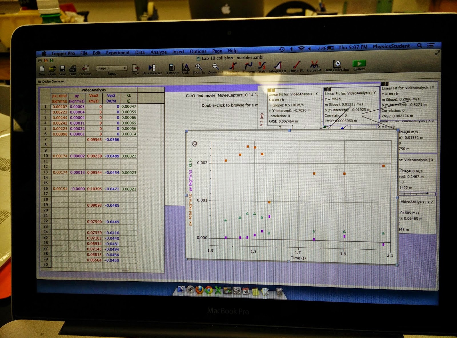
The following is the graph of the velocity, and position of the hanging mass and the elastic force of the oscillating motion:

With the measurements collected by the motion sensor and the force sensor, we were able to derive columns for kinetic energy, elastic potential energy, and gravitational potential energy.
KEm(J)=1/2*(hanging mass in kg)V^2
KEspr(J)=1/2*(mass of spring in kg/3)V^2
GPEm=MgHbottom
GPEspr=constant+(mass of spring in kg/2)*gHbottom
EPEspr=1/2k(stretched distance)^2
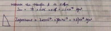
The following is the complete table with all the calculated columns:

The most right column of this table is the total energy within this oscillating spring system, which has magnitude between 4.3 to 4.4 J. This indicates that the total energy in this system is almost a constant value.
The following is the Energy(J) vs. Time(s) graphs:

We can see that total energy curve is almost a horizontal line.

Conclusion:
This experiment gives us a pretty good look at the relationship between different forms of energies within a system. We found the oscillation of the spring with hanging mass obeying the law of conservation of energy. The graph of energies versus time above shows that the potential energy decreases when the elastic energy and the kinetic energy increase, and vise versa. Through this experiment, we proved the statement of the law of conservation of energy to be true.